Graph-Based Shapes

This purely graphical shader programming solution has been designed to provide easier access to parametric modelling for people who prefer node-based modeling or are not proficient with programming or scripting. Creating a new model and selecting the New Graph option will create a <filename>.graph and a <filename>.graph.wgsl file. The .wgsl file is automatically generated from the code graph and is always updated when changes occur.

General Usage

Creating a new code graph will initialize it with the necessary nodes to render a sphere. There are two nodes that every code graph needs to have. They are essential entry and exit points for node-based parametric modeling:

• input2: This is the starting point. It represents the two input parameters to parametric modeling.
• Return: This is the node that receives the final 3D coordinates. It is important to note that the Return node requires a vec3f as an input value, so just connecting the input2 node would not work.

The code graph can be navigated with these controls:

• Move around by holding the left mouse button and dragging the mouse
• Zoom in and out with the scroll wheel
• Select nodes by left clicking them
• Select multiple nodes by holding CTRL while left clicking them
• Open a context menu with various options by pressing the right mouse button
• Create new nodes by dragging them from the nodes list on the left side into the graph
• View the generated code by clicking the button at the top-right corner

Graph-based parametric modeling is performend with nodes and connections.

Nodes

These blocks (both visually and practically) contain user-controlled data (i.e. numerical values, input connections) and internal functionality to determine the line of code to generate. Only the first part is relevant for using the code graph.

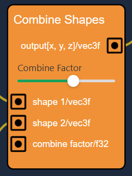
The image above shows a simple node of the graph. Every node has a title, which is written right on top (i.e. Combine Shapes). What follows are the outputs of the node on the right side. Next to the outputs the output value is described with a name and the value type to be returned seperated by a '/'. The different value types in the code graph are limited to:

• f32: a floating point number
• vec2f: a 2-dimensional vector of floating point numbers
• vec3f: a 3-dimensional vector
• vec4f: a 4-dimensional vector
• any: the type depends on the input of the node and is either one of the above
• same: the type is the same as the input type

Next there are the manual input fields, in this case the combine factor. These are fields that are defined by the user and can be changed whenever. Differently from the input slots, which will be discussed in the next session, these fields typically don't take values from other nodes.

Lastly most nodes have input slots as well. These are listed on the left side and always at the bottom of a node. Just like the outputs, the input slots have labels that work the same way. These input slots have default values and accept output values from other nodes, which will replace the default value. In this case there are shape 1, a 3-dimensional vector input, shape 2, another 3-dimensional vector input and combine factor as an alternative input method for the manual combine factor.

Connections

The yellow lines going from node to node throughout a code graph are called Connections and allow the nodes to transfer data between each other. The flow is always the same, one output from node A goes into the input of node B, so node B can access the output value from node A, but not vice versa.

The image above shows the connection between the node Sphere and Add. Looking at the input slots of Add first reveals that it accepts two inputs of any type as described above. The Sphere node has an output of the type vec3f which is a valid type for the input slot for "First Operand" of the Add node. The other input "Second Operand" is given manually in the number field and set to 3. Alternatively the "Second Operand" could also be a connection between one node and this Add node. If the Sphere node changed in any way, the Add node would immediately receive the new output data and therefore generate a different output data as well.

Code Graph Overview - Heart-Sphere example

When opening the "Math2Model" Web application for the first time a simple scene rendering a heart will open. This heart represents the "MorphHeartSphere" model in the Scene Hierarchy on the left side. Clicking on the model in the Scene Hierarchy shows the code graph of the model on the right side.

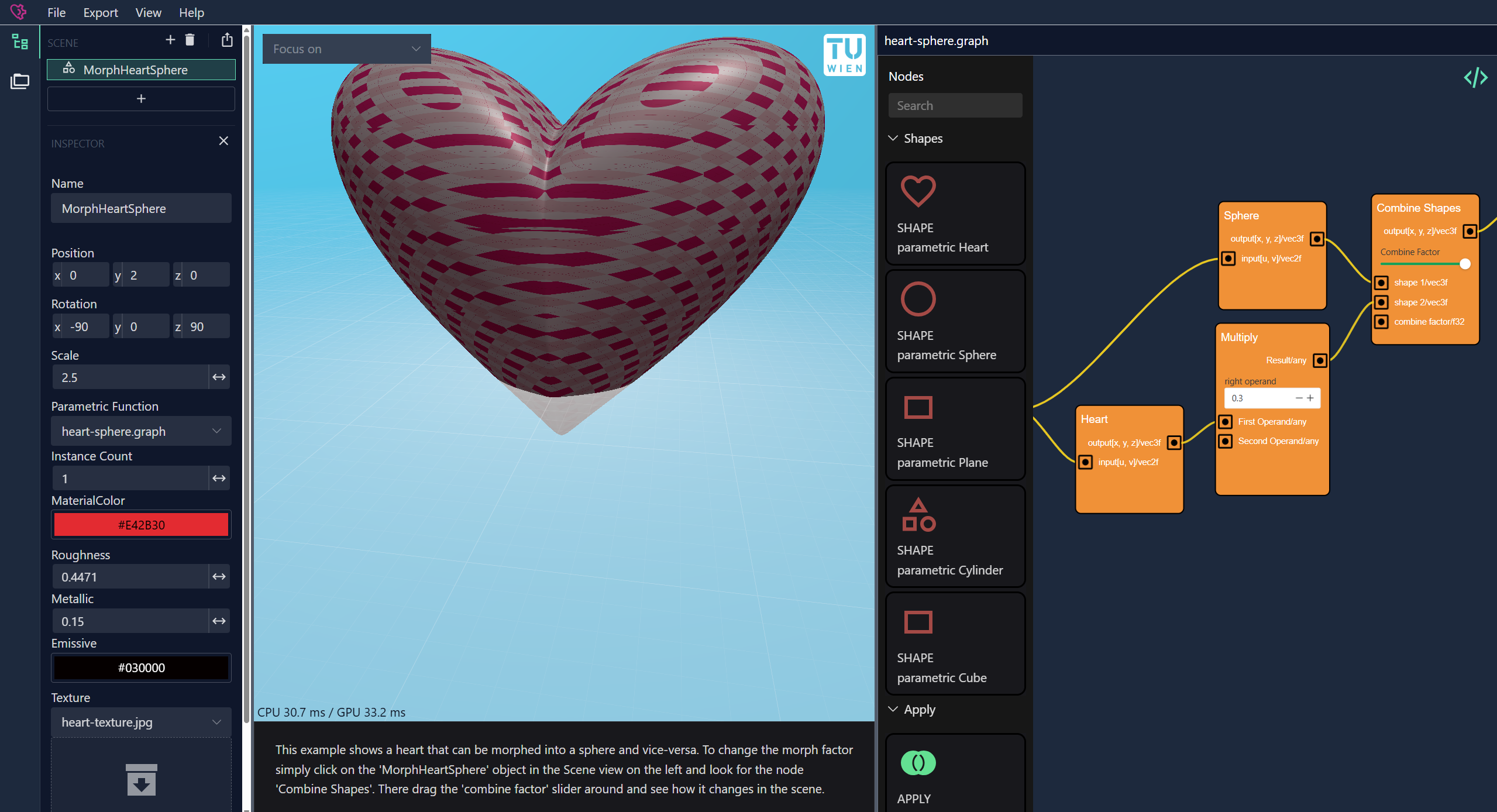
The figure above shows the state of the application after opening the code graph.

Like in every code graph, the one in the figure above starts with the input2 node, which represents the input coordinates of the plane that is parametrically shaped. This initial node is connected to the Heart and Sphere node, which can both be found under the Shapes category in the nodes list. Defining a base shape for the parametric object is common usage of code graphs. The generated code looks something like this (full code available after loading the Heart-Sphere example under heart-sphere.graph.wgsl).

var ref_831ed = Sphere(input2); // this creates a vec3f reference to the value of Sphere(input2)
var ref_fd7fa = Heart(input2); // this creates a vec3f reference to the value of Heart(input2)

The Shapes nodes - just like Heart or Sphere - typically transform a two-dimensional input into a three-dimensional output which can be directly connected to the Return value on the Return node.

After scaling down the Heart shape it is then connected to the Combine Shapes node. This node interpolates between the inputs of "shape 1" and "shape 2" using the "combine factor" as the interpolation factor. The result of this node is being returned. Dragging around the "combine factor" slider shows immediate results.